Networks

After studying this section you should be able to:

understand flows in networks and be able to find the maximum flow for a network involving multiple sources and sinks
understand the travelling salesman problem and calculate upper and lower bounds for the total distance

Flows in networks

The flows referred to may be flows of liquids, gases or any other measurable quantities. The edges may represent such things as pipes, wires or roads that carry the quantities between the points identified as vertices.

A typical vertex has a flow into it and a flow out of it. The exceptions are a source vertex which has no input and a sink vertex which has no output.

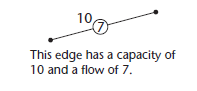
Each edge of the network has a capacity which represents the maximum possible flow along

that edge. In the usual notation, the capacity is written next to the edge and the flow is shown in a circle.

The set of flows for a network is feasible if:

The total output from all source vertices is equal to the total input for all sink vertices.
The input for each vertex other than a source or sink vertex is equal to its output.
The flow along each edge is less than or equal to its capacity.

A cut divides the vertices into two sets, one set containing the source and the other containing the sink.

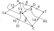
The capacity of a cut is equal to the sum of the capacities of the edges that cross the cut, taken in the direction from the source set to the sink set.

In the diagram, the capacity of cut (i) is 15 + 10 = 25.

The capacity of cut (ii) is 8 +14 = 22.

Notice that, for the second cut, the capacity of 4 is not included because it does not go from the source set to the sink set.

Be careful to add the capacities and not the flows.

The maximum flow - minimum cut theorem

The maximum flow–minimum cut theorem states that the maximum value of the flow through a network is equal to the capacity of the minimum cut. (This is a little bit like saying that a chain is only as strong as its weakest link.)

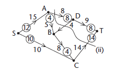
It follows from the theorem that if you find a flow that is equal to the capacity of some cut then it must be the maximum flow that can be established through the network.

For example, the capacity of cut (ii) for this network has already been found to be 22. The circled figures show one way of achieving this flow and the theorem now tells us that this must be the maximum possible flow through the network.

Flow augmentation

Once an initial flow has been established through a network it is useful to know the extent to which the flow along any edge may be altered in either direction.

This is labelled as excess capacity and back capacity on each edge as shown. It may be possible to augment the flow through the network by making use of this flexibility along a path from the source vertex to the sink vertex.

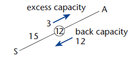
Such a path is called a flow-augmenting path.

A saturated edge is one where the flow is equal to the capacity.

An algorithm for finding the maximum flow through a network by augmentation is:

Step 1 Find an initial flow by inspection.
Step 2 Label the excess capacity and back capacity for each edge.
Step 3 Search for a flow-augmenting path. If one can be found then increase the flow along the path by the maximum amount that remains feasible.
Step 4 Repeat steps 2 and 3 until no flow-augmenting path may be found.

Multiple sources and sinks

A network may have several sources S₁, S₂, … and several sinks T₁, T₂, … but the methods described in this section can still be applied through the use of a supersource and a supersink. A supersource S is an extra node, added to the network, that acts as a source for each of the original sources. Similarly, a supersink T is a node, added to the network, that acts as a sink for each of the original sinks.

Example

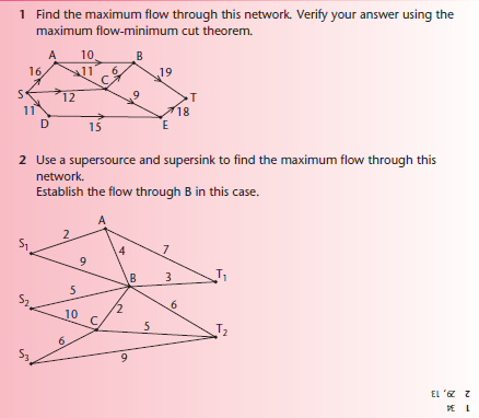
The network below shows two sources S₁ and S₂ and two sinks T₁ and T₂.

Find the maximum flow through the network and state any flow-augmenting paths.

Explain why the flow is maximal.

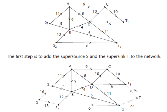
The usual convention is to use dotted lines for the edges linking S and T to the network.

The capacities on the edges SS₁ and SS₂ have been chosen to support the maximum possible flows from S₁ and S₂. Similarly, the capacities on the edges T₁T and T₂T have been chosen to support the maximum flows into T₁ and T₂.

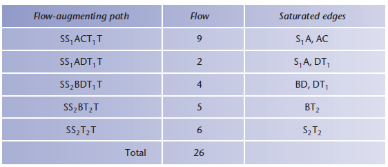
The diagram also shows a cut with capacity 11 + 4 + 5 +6 + 26.

A flow of 26 can be achieved as shown in the table.

The flows on the flow-augmenting paths are shown circled on the network below.

The flow of 26 is maximal since it equals the capacity of the cut (maximum flow minimum cut theorem).

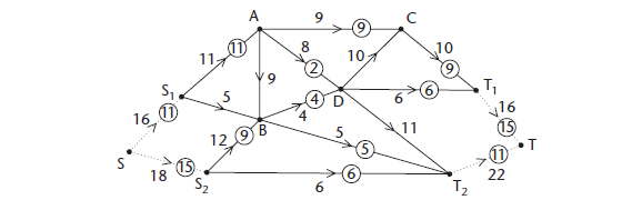
Note that each of the edges on the minimum cut is saturated. This will always be the case.

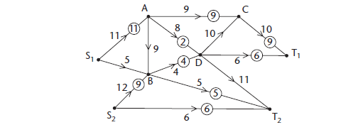
The final stage is to remove the supersource and supersink, along with the extra arcs, to show the maximum flow pattern for the original network.

The travelling salesman problem

The travelling salesman problem (TSP) is the problem of finding a route of minimum distance that visits every vertex and returns to the start vertex. For a small network it is possible to produce an exhaustive list of all possible routes and choose the one that minimises the total distance. For a large network an exhaustive check is not feasible, even with a computer, because the number of possible routes grows so rapidly.

It is useful to know within what limits the total distance must lie and there are algorithms that can be used for this purpose.

This is based on the classic situation of a salesman who wishes to visit a number of towns and return home using the shortest possible route.

Finding an upper bound

KEY POINT - An upper bound for the total distance involved in the travelling salesman problem is given by twice the minimum spanning tree.

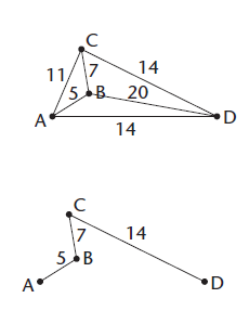
The minimum spanning tree (MST) for the network ABCD may be found using Prim’s algorithm or Kruskal’s algorithm.

The total length of the MST is 5 + 7 +14 = 26.

An upper bound for the TSP is 2 X 26 = 52.

This corresponds to the route ABCDCBA.

However, an improved (smaller) upper bound can be found by using a short-cut from D directly back to A.

The route is then ABCDA and the corresponding upper bound is 40.

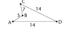
A different approach is to use the nearest neighbour algorithm ABOVE.

Step 1 Choose a starting vertex.
Step 2 Move from your present position to the nearest vertex not yet visited.
Step 3 Repeat step 2 until every vertex has been visited. Return to the start vertex.

For the network ABCD considered above, the nearest neighbour algorithm gives the same result as using the MST with a short-cut. This won’t always be the case.

Finding a lower bound

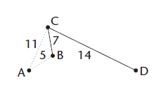
Step 1 Choose a vertex and delete it along with all of the edges connected to it.
Step 2 Find a minimum spanning tree for the remaining part of the network.
Step 3 Add the length of the MST to the lengths of the two shortest deleted edges

The value found at step 3 is a lower bound for the travelling salesman problem.

It may be possible to find a better (larger) lower bound by choosing to delete a different vertex initially and repeating the process.

Using the network ABCD again and deleting A gives the minimum spanning tree BCD of length 7 + 14 + 21. Adding the two shortest deleted lengths gives a lower bound of 37.

KEY POINTS FROM AS: Revise Prim’s algorithm and Kruskal’s algorithm

NOTE: In some cases you might be able to find more than one short-cut that will enable you to reduce the upper bound.
Deleting D to start with gives a lower bound of 40. This corresponds to a cycle ABCDA and so represents the solution of the TSP.

PROGRESS CHECK

Log in